Cheeger problems

\[\renewcommand{\div}{\operatorname{div}} \newcommand{\bsig}{\boldsymbol{\sigma}}\]

Dual problem

The Cheeger problem dual formulation reads as:

\[\begin{split}\begin{equation} \begin{array}{rl} \displaystyle{\sup_{\lambda\in \mathbb{R}, \bsig\in W}} & \displaystyle{\lambda} \\ \text{s.t.} & \lambda f = \div\bsig \quad \text{in }\Omega \\ & \|\bsig\|_2 \leq 1 \end{array} \label{Cheeger-dual} \end{equation}\end{split}\]

A natural discretization strategy for such a problem is to use \(H(\div)\)-conforming elements such as the Raviart-Thomas element \(RT_1\). Two minimization variables are therefore defined: \(\lambda\) belonging to a scalar Real function space and \(\bsig \in RT_1\). Since for \(\bsig \in RT_1\), \(\div \bsig \in \mathbb{P}^0\), we write the constraint equation using \(\mathbb{P}^0\) Lagrange multipliers:

Implementation

#!/usr/bin/env python3
# -*- coding: utf-8 -*-
"""
Dual convex optimization formulation of the Cheeger problem.

Discretization of the dual field sigma using Raviart-Thomas elements.

@author: Jeremy Bleyer, Ecole des Ponts ParisTech,
Laboratoire Navier (ENPC, Univ Gustave Eiffel, CNRS, UMR 8205)
@email: jeremy.bleyer@enpc.fr
"""
from ufl import div
from dolfin import UnitSquareMesh, FunctionSpace, Constant, dx, plot
from fenics_optim import MosekProblem, L2Ball
import matplotlib.pyplot as plt

N = 25
mesh = UnitSquareMesh(N, N, "crossed")

VRT = FunctionSpace(mesh, "RT", 1)
R = FunctionSpace(mesh, "Real", 0)
# FunctionSpace for the Lagrange multiplier associated with "constraint"
VDG0 = FunctionSpace(mesh, "DG", 0)

prob = MosekProblem("Cheeger dual")
lamb, sig = prob.add_var([R, VRT])

f = Constant(1.0)


def constraint(u):
    """Equilibrium constraint."""
    return (lamb * f - div(sig)) * u * dx


prob.add_eq_constraint(VDG0, A=constraint, name="u")

# We add the L2-Ball constraint ||sigma||_2 <= 1
F = L2Ball(sig, quadrature_scheme="vertex")
prob.add_convex_term(F)

# objective function is c(lambda, sigma) = lambda = [1, 0]*(lambda, sigma)
prob.add_obj_func(lamb * dx)

prob.parameters["presolve"] = True

# we enforce maximization
prob.optimize(sense="max")

# Dual variables are in prob.y
# The first constraint defined being lambda*f+div(sig)=0
# we get its associated Lagrange multiplier u using its name
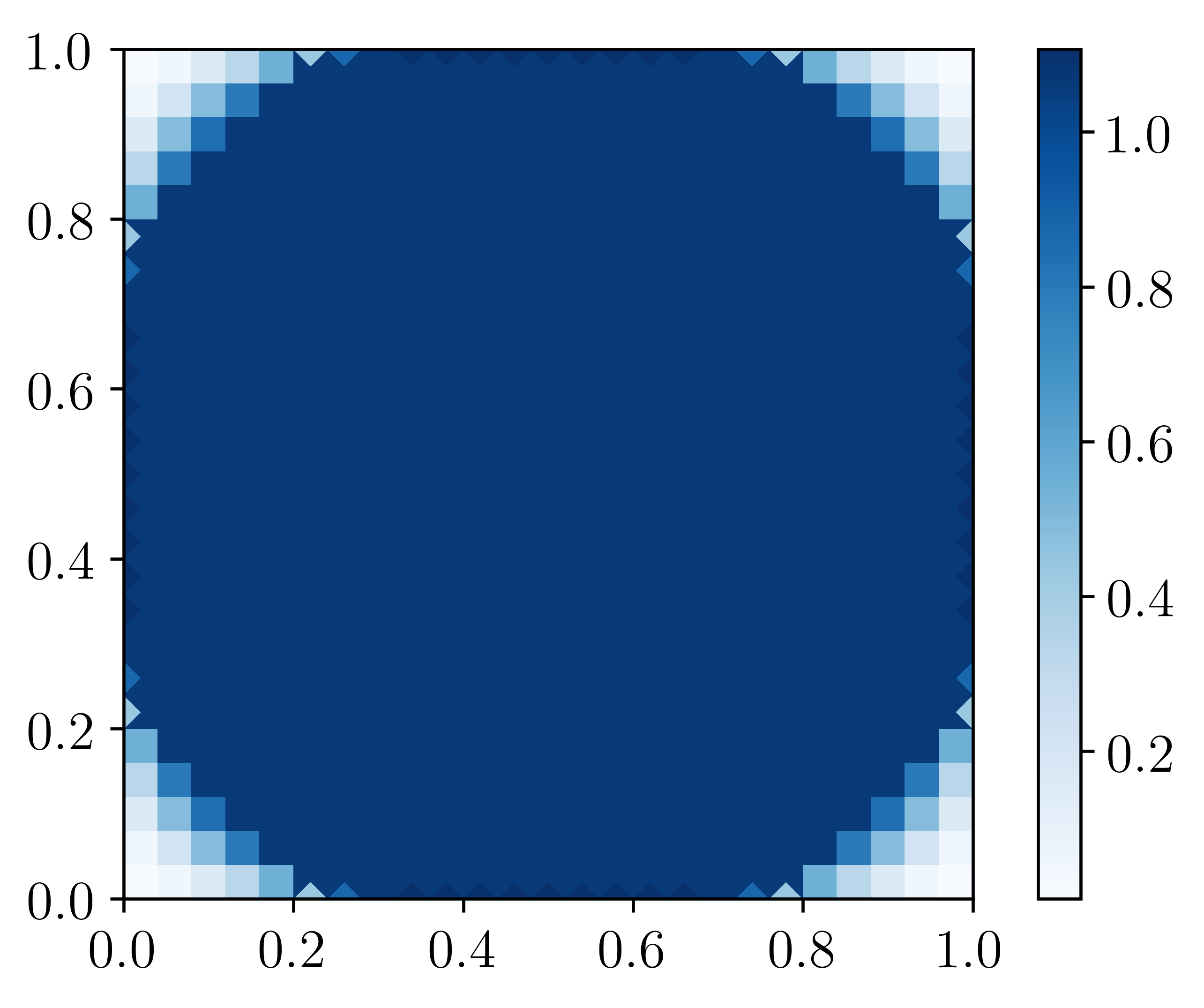
u = prob.get_lagrange_multiplier("u")

plt.figure()
plot(u, cmap="Blues")
plt.show()