Hele-Shaw flow of a viscoplastic fluid

Hele-Shaw problem

\(\newcommand{\bU}{\boldsymbol{U}} \newcommand{\bA}{\boldsymbol{A}} \newcommand{\bG}{\boldsymbol{G}} \newcommand{\bI}{\boldsymbol{I}} \newcommand{\bu}{\boldsymbol{u}} \newcommand{\bd}{\boldsymbol{d}} \newcommand{\be}{\boldsymbol{e}} \newcommand{\br}{\boldsymbol{r}} \newcommand{\bs}{\boldsymbol{s}} \newcommand{\bx}{\boldsymbol{x}} \newcommand{\by}{\boldsymbol{y}} \newcommand{\bsig}{\boldsymbol{\sigma}} \newcommand{\btau}{\boldsymbol{\tau}} \newcommand{\bgamma}{\boldsymbol{\gamma}} \newcommand{\dz}{\,\text{dz}} \newcommand{\Qq}{\mathcal{Q}} \renewcommand{\div}{\operatorname{div}} \newcommand{\dS}{\text{dS}} \newcommand{\bn}{\boldsymbol{n}}\)

A Hele-Shaw cell consists of two plates which are extremely close to each other in order to induce a bidimensional flow. This serves as a model for flows in porous media. Each plate is located at a position \(z=\pm H(x,y)\) (symmetric configuration with respect to \(z=0\)).

Although the flow is macroscopically two-dimensional and can be described by a macroscopic in-plane velocity \(\bU = U_x(x,y)\be_x+U_y(x,y)\), the local three-dimensional flow \(\bu(x,y,z)\) admits a specific profile in the transverse \(z\)-direction between both plates.

In order to link the local 3D behaviour of the fluid with an effective 2D behaviour, a dimensionality reduction procedure is considered accounting for several hypotheses [HUI05, Section 7.3]:

• the transverse velocity is negligible: \(u_z\approx 0\)

• the velocity variations in the transverse directions are much larger than the in-plane variations \(\|\bu_{,x}\|,\|\bu_{,y}\| \ll \|\bu_{,z}\|\)

• a no-slip condition is assumed along both plates walls \(z=\pm H\)

• inertia and body forces can be ignored

Such a procedure is not trivial in the case of a Bingham fluid which exhibits solid and flowing regions along the transverse direction. The yield point between flowing and solid region is unknown a priori and depends upon the corresponding stress and pressure gradient.

Indeed, with the above hypotheses, one can easily show that the shear stress field varies linearly along the transverse direction as follows:

\begin{align} \bsig(x,y,z) &\approx \begin{bmatrix} 0 & 0 & \tau_x \\ 0 & 0 & \tau_y \\ \tau_x & \tau_y & 0\end{bmatrix} \\ \text{with } \btau(x,y) &= z \nabla p(x,y) \end{align}

where \(\btau(x,y,z)\) is the anti-plane shear stress vector and \(p(x,y)\) is the fluid pressure.

Determining effective potentials

The Hele-Shaw effective behaviour can be described through effective potentials, either in stress-based form as a potential function \(\Psi(\bG)\) of the pressure gradient \(\bG(x,y)=-\nabla p(x,y)\) or in velocity-based form as a potential function \(\Phi(\bU)\) of the macroscopic velocity \(\bU(x,y)\). Both potentials are dual to each other, that is they are related via Legendre-Fenchel transform \(\Psi = \Phi^*\) and we have:

\begin{equation} \bU = \partial_\bG \Psi(\bG) \quad,\quad \bG = \partial_\bU \Phi(\bU) \end{equation}

The stress-based potential for instance can be obtained from the integrated stress potential as follows:

\begin{equation} \Psi(\bG) = \dfrac{1}{2H}\int_{-H}^H \psi(\bsig(x,y,z))\dz \end{equation}

where \(\psi\) is the 3D stress-based potential of the constituting fluid.

For instance, for a Newtonian fluid, one has \(\psi(\bsig) = (\bsig:\bsig)/(4\mu)\) with \(\bd = \partial_\bsig \psi = \bsig/(2\mu)\). The corresponding effective potential is then given by:

\begin{equation} \Psi(\bG) = \int_{-H}^H \dfrac{1}{4\mu H} z^2 \bG\cdot\bG \dz = \dfrac{H^2}{6\mu} \bG\cdot\bG \end{equation}

which results in the following linear effective constitutive relation:

\begin{equation} \bU = \partial_\bG \Psi(\bG) = \dfrac{H^2}{3\mu} \bG \end{equation}

from which we recover the classical Darcy equation between two parallel plates.

Alternatively, the velocity-based potential is obtained via Legendre-Fenchel transform:

\begin{equation} \Phi(\bU) = \sup_{\bG} \{\bU\cdot\bG - \Psi(\bG)\} \end{equation}

which after standard convex duality computations yields:

\begin{equation} \begin{array}{rl} \displaystyle{\Phi(\bU) = \inf_{\bgamma(z)}} & \displaystyle{\dfrac{1}{2H}\int_{-H}^H \phi(\bd(z))\dz} \\ \text{s.t.} & \bd(z) = \begin{bmatrix} 0 & 0 & \gamma_x(z) \\ 0 & 0 & \gamma_y(z) \\ \gamma_x(z) & \gamma_y(z) & 0 \end{bmatrix} \\ & \bU + \dfrac{1}{2H}\int_{-H}^{H} z\bgamma(z)\dz = 0 \end{array} \end{equation}

In the above formulation, we see that when interpreting \(\bgamma(z)\) as the local strain rate \(\bgamma(z)=\bu_{,z}\), the constraint indeed enforces the link with the macroscopic velocity:

\begin{equation} \bU + \dfrac{1}{2H}\int_{-H}^{H} z\bu_{,z}\dz = \bU - \dfrac{1}{2H}\int_{-H}^{H} \bu\dz =0 \end{equation}

The Bingham case and its conic representation

Numerical approximation

For a Bigham fluid of viscosity \(\mu\) and yield stress \(\tau_0\), the velocity-based potential can be expressed as:

\begin{equation} \begin{array}{rl} \displaystyle{\Phi(\bU) = \inf_{\bgamma(z)}} & \displaystyle{\dfrac{1}{2H}\int_{-H}^H \left(\dfrac{\mu}{2}\|\bgamma(z)\|^2 + \tau_0\|\bgamma(z)\|\right)\dz} \\ \text{s.t.} & \displaystyle{\bU + \dfrac{1}{2H}\int_{-H}^{H} z\bgamma(z)\dz = 0} \end{array} \end{equation}

Unfortunately, there is no closed-form expression for solving the inner minimization over the \(\bgamma(z)\) field. For a practical numerical implementation, we therefore have to resort to some numerical approximation. In the following, we choose to restrict the field \(\bgamma(z)\) to a finite set of values \(\bgamma_i = \bgamma(z_i)\) at some integration points \(z_i\). The above integrals are then replaced by a numerical quadrature using such points. Moreover, we benefit from out initial assumption of a symmetric configuration so that the integral is performed over \([0;H]\) only. Introducing, the non-dimensional integration points \(\xi_i=z_i/H\) and their corresponding quadrature weights \(\omega_i\) on \([0;1]\), we finally have the following approximate potential depending on the number \(m\) of quadrature points:

\begin{equation} \begin{array}{rl} \displaystyle{\Phi_m(\bU) = \inf_{\bgamma_i}} & \displaystyle{\sum_{i=1}^m \omega_i\left(\dfrac{\mu}{2}\|\bgamma_i\|^2 + \tau_0\|\bgamma_i\|\right)} \\ \text{s.t.} & \displaystyle{\bU + H \sum_{i=1}^m \omega_i\xi_i\bgamma_i = 0} \end{array} \end{equation}

Note that such an approach has already been proposed in [BLE16] when deriving effective strength criteria of shells from the local 3D strength criterion.

Explicit conic representation

To obtain a conic form, we use the classical epigraph reformulation. Let \(i=1,\ldots,m\). Introducing \(\br^i=(r_0^i,r_1^i,r_2^i)\in \Qq_3\) such that \((r_1^i,r_2^i)=\bgamma^i\), we replace \(\tau_0\|\bgamma_i\|\) with \(\tau_0 r_0^i\) such that \(\|\bgamma_i\|\leq r_0^i\). For the quadratic term, we introduce \(\bs^i=(s_0^i,s_1^i,s_2^i)\in \Qq_3^r\) such that \(s_1^i=1\) and \(s_2^i=r_0^i\). Doing so, we benefit from the fact that it can be replaced with \(\dfrac{\mu}{2}\|\bgamma_i\|^2 \leq \dfrac{\mu}{2} (r_0^i)^2 \leq \mu s_0^i\) since we have \((r_0^i)^2=(s_2^i)^2\leq 2s_1^is_0^i=s_0^i\). We finally have:

\begin{equation} \begin{array}{rl} \displaystyle{\Phi_m(\bU) = \inf_{\bgamma_i,\br_i,\bs_i}} & \displaystyle{\sum_{i=1}^m \omega_i\left(\mu s_0^i + \tau_0r_0^i\right)} \\ \text{s.t.} & \displaystyle{\bU + H \sum_{i=1}^m \omega_i\xi_i\bgamma_i = 0} \\ & (r_1^i,r_2^i)=\bgamma^i \\ & s_1^i=1 \\ & s_2^i=r_0^i \qquad \forall i=1,\ldots,m \\ & \br^i\in \Qq_3 \\ & \bs^i \in \Qq_3^r \end{array} \end{equation}

Marginal composition of the Bingham potential

Implementing directly the above representation lacks generality since it must be repeated each time one wants to change the underlying fluid potential e.g. considering a Hershel-Bulkley fluid for instance. Instead, we can use the abstract Marginals operator which is defined as follows for any convex function \(f(\by)\), a list of linear operators \(\bA_i\) and positive coefficients \(c_i\):

\begin{equation} \begin{array}{rl} \displaystyle{f \setminus \{\bA_i,c_i\}(\bx) = \inf_{\by_i}} & \displaystyle{\sum_{i=1}^m c_i f(\by_i)} \\ \text{s.t.} & \bx = \displaystyle{\sum_{i=1}^m \bA_i \by_i} \end{array} \end{equation}

Using such an abstract operator, any Hele-Shaw potential can be obtained as the Marginals of the underlying fluid potential \(\phi(\bgamma)\) through the linear operators \(\bA_i = -H\omega_i \xi_i \bI\) and the coefficients \(c_i=\omega_i\). In the following implementation we use this strategy. Note that the Lagrange multiplier associated with the last constraint gives directly access to the pressure gradient \(\bG=\partial_\bU \Phi(\bU)\).

FEniCS implementation

Numerical implementation and results at the material point level

Let us first implement and test this behaviour at the material point level in order to compute a flow curve in the \((\bU,\bG)\) plane.

from dolfin import (
    UnitIntervalMesh,
    VectorFunctionSpace,
    Function,
    Constant,
)
from fenics_optim import (
    ConvexFunction,
    MosekProblem,
    Quad,
    RQuad,
    tail,
    dummy_variable,
    Marginals,
)
from ufl import Identity
import numpy as np
import matplotlib.pyplot as plt


class BinghamPotential(ConvexFunction):
    def __init__(self, x, mu, tau0, **kwargs):
        ConvexFunction.__init__(self, x, parameters=(mu, tau0), **kwargs)

    def conic_repr(self, X, mu, tau0):
        y = self.add_var(self.dim_x + 1, cone=Quad(self.dim_x + 1))
        z = self.add_var(3, cone=RQuad(3))
        self.add_eq_constraint(X - tail(y))
        self.add_eq_constraint(z[2] - y[0])
        self.add_eq_constraint(z[1], b=1)
        self.set_linear_term(mu * z[0] + tau0 * y[0])


def HeleShawPotential(m, H, potential):
    points, weights = np.polynomial.legendre.leggauss(m)
    # transform for integration on [0;1]
    points = (points + 1) / 2
    weights /= 2

    c_list = list(weights)
    A_list = [-H * wi * zi * Identity(2) for (zi, wi) in zip(points, weights)]
    return lambda U: Marginals(
        potential,
        A_list,
        U,
        c_list=c_list,
        lagrange_multiplier_name="Pressure gradient",
    )


def compute_flow(U_d, m, tau0):
    H = Constant(1.0)
    mu = Constant(1.0)

    mesh = UnitIntervalMesh(1)
    V = VectorFunctionSpace(mesh, "R", 0, dim=2)

    prob = MosekProblem("Hele Shaw flow")
    U_v = Function(V)
    U_v.vector()[0] = U_d
    U = prob.add_var(V, lx=U_v, ux=U_v)

    dummy = dummy_variable(2, mesh)
    bingham_pot = BinghamPotential(dummy, mu, tau0)
    hele_shaw_pot = HeleShawPotential(m, H, bingham_pot)

    prob.add_convex_term(hele_shaw_pot(U))
    prob.parameters["log_level"] = 0
    prob.optimize()
    G = -prob.get_lagrange_multiplier("Pressure gradient").vector()[0]
    return G


def compute_flow_curve(m, tau0):
    Ulist = np.concatenate((np.array([0]), np.linspace(0.00001, 0.2 * float(tau0), 20)))
    return Ulist, np.array([compute_flow(ui, m, tau0) for ui in Ulist])

tau0 = Constant(1.0)

G = {}
for m in [2, 3, 4, 6]:
    print(f"Computation with {m} quadrature points...")
    Ulist, G[m] = compute_flow_curve(m, tau0)

Computation with 2 quadrature points...
Computation with 3 quadrature points...
Computation with 4 quadrature points...
Computation with 6 quadrature points...

We now compare the obtained flow curves with the analytical solution provided in [HUI05, eq. (7.3.36)]:

\begin{align} \bU &= \dfrac{H^2}{3\mu}\left(1 - \dfrac{3}{2\|\bG\|} + \dfrac{1}{2\|\bG\|^3} \right)\bG \quad \text{ if }\|\bG\|>\tau_0/H \\ \bU &= 0 \text{ otherwise} \end{align}

Ub = Ulist / float(tau0)
G_an = np.linspace(0, 2, 200)
U_an = np.zeros_like(G_an)
Gan_r = G_an[G_an > 1]
U_an[G_an > 1] = Gan_r / 3 * (1 - 3 / 2 / Gan_r + 1 / 2 / Gan_r ** 3)

i = 1
plt.figure(figsize=(10, 10))
for (m, Gm) in G.items():
    plt.subplot(2, 2, i)
    plt.plot(U_an, G_an, "-k", label="exact")
    plt.plot(Ub, Gm / float(tau0), f"-C{i-1}", linewidth=1.5, label=f"$m={m}$")
    plt.xlim(-0.001, 0.2)
    plt.ylim(0, 2.0)
    plt.xlabel(r"$\mu U /(\tau_0 H)$", fontsize=16)
    plt.ylabel(r"$GH/\tau_0$", fontsize=16)
    plt.legend(loc="right")
    plt.tight_layout()
    i += 1
plt.show()

findfont: Font family ['serif'] not found. Falling back to DejaVu Sans.

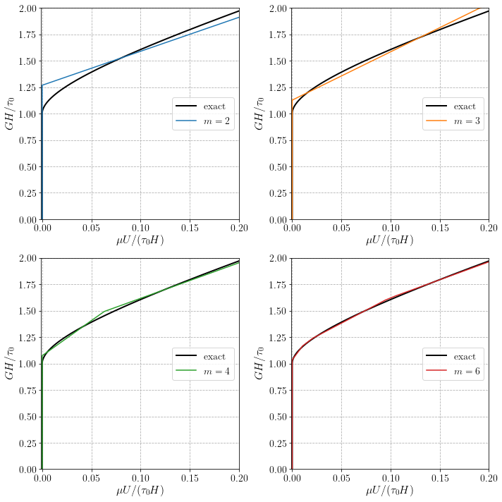
One can see that with \(m=2\) quadrature points, the behaviour resembles that of a Bingham fluid with an overestimated yield stress and an underestimated asymptotic regime. Introducing more points enables to approach the non-linear black curve with a piecewise linear curve of better quality. The choice \(m=4\) in particular is already extremely satisfying.

Flow in a random medium

Flow equations and variational principle

We now consider the Hele-Shaw flow on some domain \(\Omega\). The main unknowns for this problem are the filtration velocity \(\bU\) and the pressure field \(p\). They must satisfy the balance equation and mass conservation condition:

\begin{align} \nabla p &= 0 \quad \text{in } \Omega\\ \div\bU &= 0\quad \text{in } \Omega \end{align}

and they are related through the Hele-Shaw potential:

\begin{equation} \bG = -\nabla p = \partial_\bU \Phi(\bU) \end{equation}

along with some boundary conditions on pressure or velocity:

\begin{align} p &= p_0 &\text{ on } \partial\Omega_D \\ \bU\cdot \bn &= q &\text{ on } \partial\Omega_N \end{align}

where \(\bn\) is the outward unit normal, \(p_0\) and imposed pressure and \(q\) an imposed flux.

One can then easily see that the above equations can be derived from the following filtration velocity variational principle:

\begin{equation} \begin{array}{rl} \displaystyle{\min_{\bU}} &\displaystyle{ \int_{\Omega}\Phi(\bU)\text{d}\Omega - \int_{\partial\Omega_D} p_0 \bU\cdot\bn \dS}\\ \text{s.t.} & \div\bU = 0 \\ & \bU\cdot\bn = q\text{ on } \partial\Omega_N \end{array} \end{equation}

with the pressure field being obtained from the Lagrange multiplier associated with the mass conservation equation.

A random medium setting

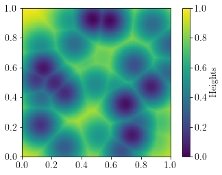
We consider here a unit square domain \(\Omega = [0;1]\times[0;1]\), subjected to \(\bU\cdot \bn=0\) on the bottom and top surfaces and imposed pressure \(p=0\) on the left boundary and \(p=p_\text{out}\) on the right boundary, mimicking an imposed macroscopic pressure gradient \(\overline{G} = p_\text{out}/L\) with \(L=1\) here. The Hele-Shaw cell consists of a heights distribution \(H(x,y)\) which is randomly generated through the piecewise combination of Gaussian profiles centered around random seed points. The field of heights is represented on a DG-0 space which will also be used to discretize the pressure field.

from dolfin import (
    UnitSquareMesh,
    FunctionSpace,
    DirichletBC,
    plot,
    dx,
    assemble,
    CompiledSubDomain,
    MeshFunction,
    FacetNormal,
    Measure,
)
from ufl import div, dot

mu, tau0 = Constant(1.0), Constant(1.0)
p_out = Constant(2.0)

N = 40
mesh = UnitSquareMesh(N, N, "crossed")


def generate_random_heights(x, Nc, R):
    """
    Generate random heights from an array of coordinates x.

    Nc denotes the number of random seed points.
    R denotes the corresponding radius size around each seed.
    """
    np.random.seed(15012017)
    centers = np.random.rand(Nc, 2)
    ampl = np.random.rand(Nc)

    res = np.zeros((x.shape[0], centers.shape[0]))
    for i, c in enumerate(centers):
        dist2 = (x[:, 0] - c[0]) ** 2 + (x[:, 1] - c[1]) ** 2
        res[:, i] = ampl[i] * np.exp(-(dist2) / R ** 2)
    return 1 - np.max(res, axis=1)


# P0 interpolation for pressure (Lagrange multiplier)
Vp = FunctionSpace(mesh, "DG", 0)

x = Vp.tabulate_dof_coordinates()
H = Function(Vp, name="Heights")
H.vector()[:] = generate_random_heights(x, 50, 0.15)

pl = plot(H, vmin=0, vmax=1)
cbar = plt.colorbar(pl)
plt.savefig("heights.png", dpi=300)
plt.show()

The velocity field is discretized using a Brezzi-Douglas-Marini space of degree \(k=1\), the pressure field being a discontinous function of degree \(k-1=0\), following the mixed Poisson demo. The mass conservation equation \(\operatorname{div}(\bU)=0\) is enforced weakly using the pressure as a Lagrange multiplier.

prob = MosekProblem("Viscoplastic fluid")

# BDM interpolation for velocity
V = FunctionSpace(mesh, "BDM", 1)

bc = DirichletBC(V, Constant((0.0, 0.0)), "near(x[1],0) || near(x[1], 1)")

U = prob.add_var(V, bc=bc)


def mass_conserv(p):
    """Mass conservation condition."""
    return p * div(U) * dx


prob.add_eq_constraint(Vp, mass_conserv)

As mentioned before, the Hele-Shaw potential is defined from the constitutive fluid potential. Here, a dummy variable of size 2 is created in order to define the Bingham fluid potential. An in-plane quadrature of degree 2 is used here. The Hele-Shaw potential is then added to the problem.

dummy = dummy_variable(2, mesh)
bingham_pot = BinghamPotential(dummy, mu, tau0, degree=2)

ngauss = 4
hele_shaw_pot = HeleShawPotential(ngauss, H, bingham_pot)

prob.add_convex_term(hele_shaw_pot(U))

Finally, we add the linear objective term corresponding to an imposed pressure \(p_{out}\) on the right boundary. We first identify the latter with some mesh tag and pass the facets mesh function to the integration measure.

outlet = CompiledSubDomain("near(x[0], 1)")
facets = MeshFunction("size_t", mesh, 1)
outlet.mark(facets, 1)
ds = Measure("ds", subdomain_data=facets)
n = FacetNormal(mesh)
prob.add_obj_func(-p_out * dot(U, n) * ds(1))

prob.optimize();

---------------------------------------------------------------------------
NameError                                 Traceback (most recent call last)
<ipython-input-5-923c9b2dd3d3> in <module>
      4 ds = Measure("ds", subdomain_data=facets)
      5 n = FacetNormal(mesh)
----> 6 prob.add_obj_func(-p_out * dot(U, n) * ds(1))
      7
      8 prob.optimize();

NameError: name 'prob' is not defined

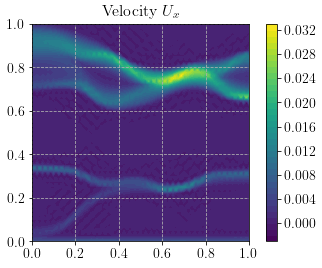
The local velocity is always zero if the applied pressure is below a certain threshold and above this threshold, the flow starts occurring in localized channels only. For higher pressure gradients, the flow then resembles that of a classical Newtonian fluid.

pl = plot(U[0])
cbar = plt.colorbar(pl)
plt.title(r"Velocity $U_x$", fontsize=16)
plt.savefig(f"velocity_p_out_{float(p_out)}.png", dpi=300)
plt.show()
print("Average velocity:", assemble(U[0] * dx))

Average velocity: 0.002216573034447165

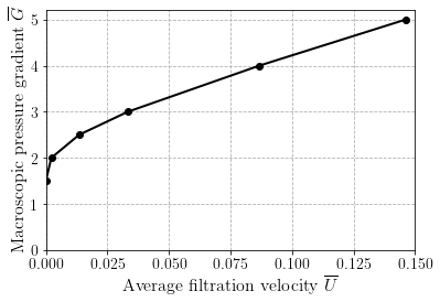
The resulting apparent flow curve between the average filtration velocity \(\overline{\bU}=\dfrac{1}{|\Omega|}\int_\Omega \bU \text{d}\Omega\) and the imposed pressure gradient \(\overline{\bG}\) is very similar to the Hele-Shaw consitutive law itself:

results = np.loadtxt("results.csv", skiprows=1, delimiter=",")
plt.plot(results[:, 0], results[:, 1], "-ok")
plt.ylim(0, 5.2)
plt.xlabel(r"Average filtration velocity $\overline{U}$", fontsize=16)
plt.ylabel(r"Macroscopic pressure gradient $\overline{G}$", fontsize=16)
plt.show()

References

[HUI05] Huilgol, R. R. (2015). Fluid mechanics of viscoplasticity. Berlin: Springer.

[BLE16] Bleyer, J., & De Buhan, P. (2016). A numerical approach to the yield strength of shell structures. European Journal of Mechanics-A/Solids, 59, 178-194.