Obstacle problem

\[\renewcommand{\div}{\operatorname{div}} \newcommand{\bsig}{\boldsymbol{\sigma}}\]

Implementation

#!/usr/bin/env python3
# -*- coding: utf-8 -*-
"""
Obstacle problem solved with fenics_optim.

@author: Jeremy Bleyer, Ecole des Ponts ParisTech,
Laboratoire Navier (ENPC, Univ Gustave Eiffel, CNRS, UMR 8205)
@email: jeremy.bleyer@enpc.fr
"""
from ufl import dot, grad
from dolfin import (
    UnitSquareMesh,
    FunctionSpace,
    Function,
    DirichletBC,
    Constant,
    Expression,
    dx,
    plot,
)
from fenics_optim import MosekProblem, QuadraticTerm
import numpy as np
import matplotlib.pyplot as plt

N = 100
mesh = UnitSquareMesh(N, N, "crossed")
V = FunctionSpace(mesh, "CG", 1)

bc = DirichletBC(V, Constant(0), "on_boundary")

load = Constant(-5)
hmean = -0.1
ampl = 0.01
k1, k2 = 2, 8
obstacle = Function(V)
obstacle.interpolate(
    Expression(
        "h+a*sin(2*pi*k1*x[0])*cos(2*pi*k1*x[1])*sin(2*pi*k2*x[0])*cos(2*pi*k2*x[1])",
        h=hmean,
        a=ampl,
        k1=k1,
        k2=k2,
        degree=2,
    )
)

prob = MosekProblem("Obstacle problem")
u = prob.add_var(V, bc=bc, lx=obstacle)
prob.add_obj_func(-dot(load, u) * dx)


F = QuadraticTerm(grad(u), degree=0)
prob.add_convex_term(F)

prob.parameters["presolve"] = True
prob.optimize()

x = np.linspace(0, 1, 200)
y = 0.5
U = [u(xi, y) for xi in x]
plt.figure(1)
plt.plot(
    x,
    hmean
    + ampl
    * np.sin(2 * np.pi * k1 * x)
    * np.sin(2 * np.pi * k2 * x)
    * np.cos(2 * np.pi * k1 * y)
    * np.cos(2 * np.pi * k2 * y),
    linewidth=2,
    label="obstacle",
)
plt.plot(x, U, linewidth=1.0, label="membrane")
plt.legend()
plt.xlabel("$x$ coordinate")
plt.ylabel("Displacement")
plt.show()

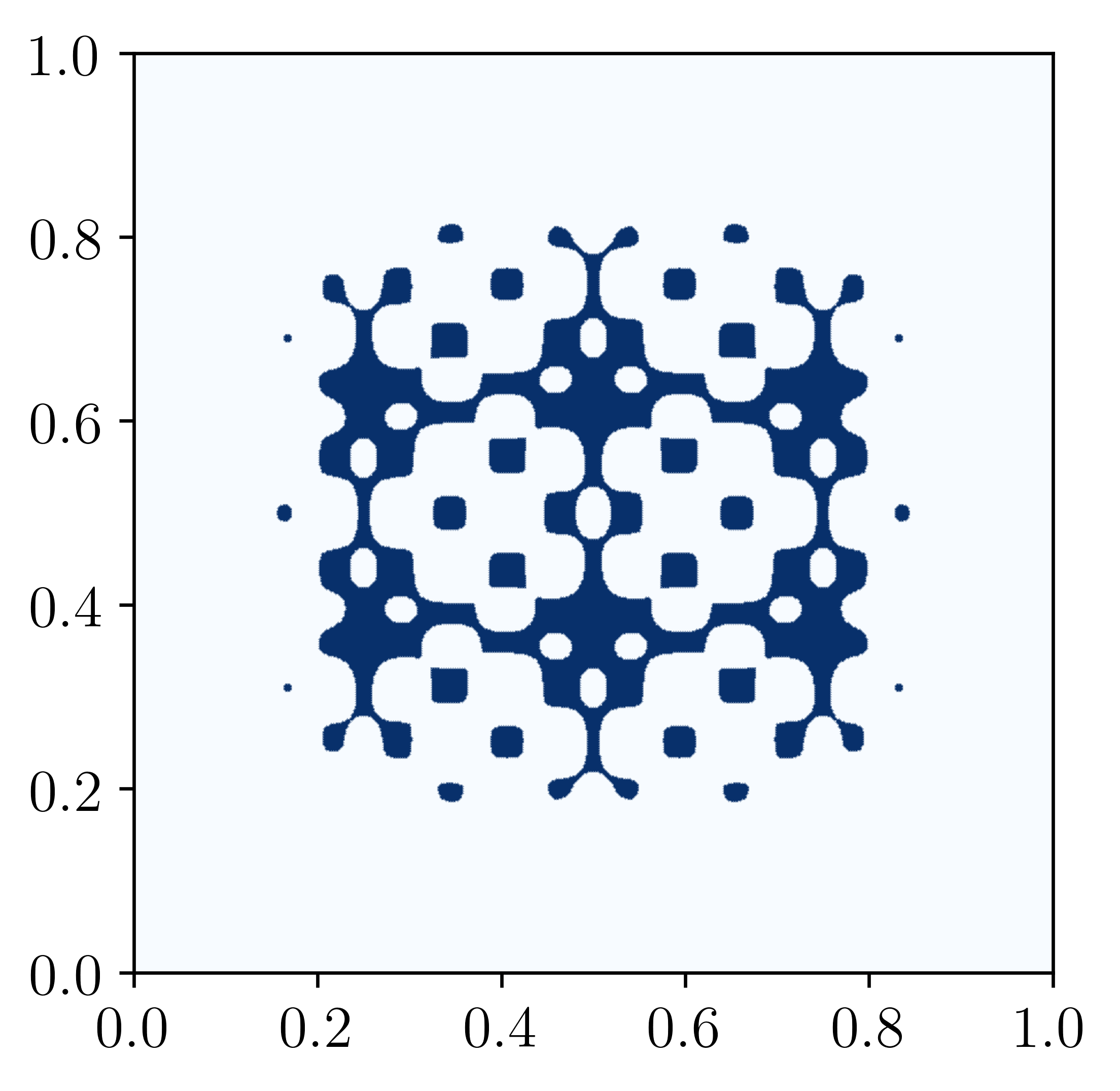
plot(u)
plt.show()